Find out how a student has developed an innovative model for detect transaction fraud and combat cyberattacks in this master's thesis.
Currently, with the advances in technology and Internet access, payment methods have evolved, and there are now different ways to make payments, whether in person or online. Just as payment methods have changed to adapt to the needs and preferences of customers and businesses, the Cybercriminals have also been evolving. Despite the various security measures adopted by financial institutions, the payment fraud It's a problem we face every day.
The financial institutions and payment service providers must evolve in tandem with the sector's needs, making use of emerging technology and the availability of data to implement security measures and establish measures for early fraud detection.
Development of a Model for Detecting Fraud in Credit Card Transactions
This interesting master's thesis, prepared Magaly Fonseca A former student of the Master's in Big Data and Business Analytics at Structuralia takes a deeper look at this topic—which is so important today—by creating a «Model for Detecting Fraud in Credit Card Transactions.».
1. Choosing a Dataset
For the preparation of this master's thesis A dataset was selected, from those available on the page Kaggle, which contains data that can be used to train a machine learning model capable of detecting cases of fraud in transactions. The chosen dataset is called card_transdata which contains information on credit card transactions.
The dataset is a file with a .csv extension and It consists of 8 columns. Described below:
- Distance_from_home: the distance from home to the location where the transaction took place.
- Distance_from_last_transaction: indicates the distance between the transaction point and the last recorded transaction—that is, the previous transaction.
- Radio_to_median_purchase_price: It is the ratio of the transaction amount to the customer's average purchase price.
- Repeat_retailer: Enter 1 if the transaction was made at the same retailer, and 0 if not.
- Used_chip: In this column, a 1 indicates that the credit card chip was used for the transaction, and a 0 indicates that it was not used.
- Used_pin_number: In this field, enter 1 if the PIN was used in the transaction, and 0 otherwise.
- Online_order: It is marked with a 1 if the transaction corresponds to an online order and with a 0 if it does not.
- Fraud: Indicates whether the transaction was flagged as fraudulent or not, just like the previous columns, with a value of 1 for fraudulent transactions and 0 for non-fraudulent ones.
2. ETL with Trifacta
For the data extraction, processing, and loading (ETL) process the tool is used Trifacta. To start the process, load the card_transdata.csv dataset into the tool and create the flow with the name “transaction data”.
The first step in the transformation process is to data profiling, in order to gain a thorough understanding of the dataset's content and verify the quality of the data, with the goal of determining the transformations that need to be performed in order to work with the data and obtain reliable results.
As shown in the image above, the data in the 8 columns of the dataset is of good quality, since the indicator bar is green in all cases, which means that the data is correct, matches the cell format, and contains no invalid or empty values. It can also be seen that the dataset contains two types of data: integers and decimals. Therefore, we proceed to complete the ETL process by running the job in Trifacta to obtain the dataset and move on to the analytical phase.
3. Statistical Study
An important part of working with data is understanding it and performing an analytical study that will allow us to make the best decisions regarding their treatment; for this process, the analysis was conducted in Python.
1. EDA Analysis
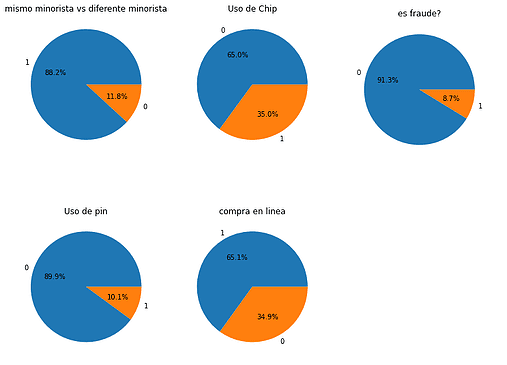
Figure 2. Graphs of the categorical variables.
As shown in the graphs, it can be seen that the 88.2% of transactions were made at the same retailer as the previous purchase. In the The chip was used for 35% transactions. The PIN was used for 10.1% of purchases, and 65.1% of transactions were online purchases. Finally, the 8.7% of transactions are fraudulent.
Box plots are created for the continuous variables to examine the distribution of the data for those variables:
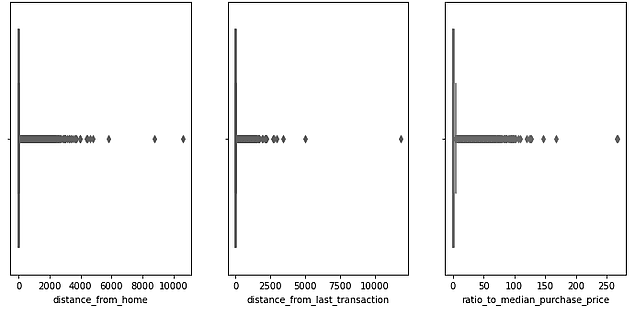
Figure 3. Box plot of the continuous variables.
For all three variables, outliers can be observed that stand out from the rest of the data when considering the variable descriptions, namely: distance from home, distance from the last transaction, and ratio relative to the average purchase amount; Furthermore, given that the goal is to train a model that predicts whether a transaction is fraudulent or not, these outliers could indicate fraudulent activity; therefore, it is determined that they should be retained.
2. Correlation Study
An important part of the analysis is conducting a correlation study to determine whether there is a relationship between the different variables in the dataset. Since the dataset contains both continuous and categorical variables, we use Spearman’s correlation method, which can be applied to both types of variables:
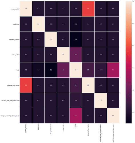
Figure 4. Correlation of the variables
The result shows a strong correlationn (0.6) between the variables “distance from home” and “whether the purchase was made at the same retailer.” Furthermore, we can see a breakdown of the variables that influence the variable of interest (fraud), where the ratio relative to the average purchase amount is the variable most strongly correlated with fraud (0.3)—although the value is not particularly high— followed by the “online purchase” variable at 0.2 and “distance from home” at 0.1. An important point emerges from this analysis: two variables show a negative correlation with fraud—chip use and PIN use—both with a value of -0.1. This could be interpreted to mean that the use of these two security methods is effective in preventing fraud in transactions.
As the final step in the statistical analysis, hypothesis tests (ANOVA) are conducted to determine whether or not the variables influence our variable of interest, which is fraud. The results are shown below:
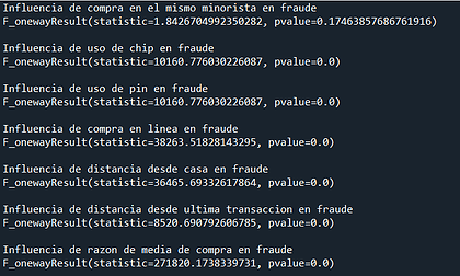
Figure 5. ANOVA Results
As can be seen, the only variable with a value greater than 0.05 is whether the purchase was made at the same retailer; therefore, the null hypothesis that the variable is influential is rejected. The remaining variables are indeed influential.
4. Visualization
Once the ETL process and the statistical analysis of the available data have been completed, the dataset is loaded into PowerBI to create a dashboard that displays the available information:
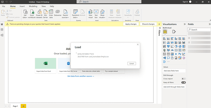
Figure 6. Loading the dataset into PowerBI.
Once the dataset has been loaded, we proceed to perform some data transformations, just to make it easier to see, these transformations apply to the data type of columns containing Boolean values; they are converted from 0 and 1 to the “true/false” type, and in the case of the Fraud Column The data type is changed to text, and the 0s are replaced with the word “no” and the 1s with “yes.” It should be noted that these transformations are performed solely to facilitate visualization; they do not modify the data source (the dataset).
Using the transformations described above, we proceed to create the dashboard with the information relevant to the case study:
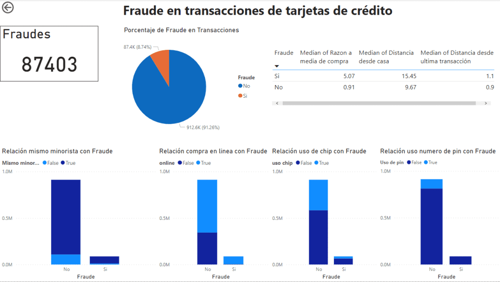
On the dashboard, you can see how Key figure: the total number of cases of fraud detected, which corresponds to 87,403 cases; this represents the 8,741 TP3T transactions, which is clearly visible in the pie chart.
In addition, a table is provided that compares the medians of the numerical variables for fraud cases versus non-fraud cases; this table shows a significant difference in the medians of the variable “ratio relative to the average purchase price””in the cases of fraud (5.07) compared to the non-fraudulent transactions (0.91); there is also a significant difference in the medians of the variable “”distance from home", since in cases of fraud the median is much higher than in cases of non-fraud; whereas for the variable “time since the last transaction,” the difference between the medians is not significant (0.2).
Finally, the following are shown: 4 bar charts, one for each Boolean variable related to the "fraud" variable. It is easy to see from these that, in cases of fraud, most of the transactions were carried out on the same retail, it is also evident that the largest proportion of fraud cases occurred in online shopping. Furthermore, it is evident that security measures such as the use of a chip and a PIN are effective in preventing fraud, with the use of a PIN being the most effective.
5. Building a Fraud Detection Model
With the goal of conducting a fraud detection model, which would be a model of classification learning. First, we determine the variables to be used. As established at the end of the statistical analysis, the variables that influence whether a transaction is fraudulent or not are all of them—except for whether the purchase was made at the same retailer. Furthermore, this variable had a high correlation with the “distance from home” variable, so only one of them should be used; this provides yet another reason to exclude the variable. “repeat_retailer”.
1. Definition of input and output variables.
Based on the information above, the input and output variables are defined as the first step in building the model; the training and test datasets are also defined, with the test set comprising 30% of the data; in addition, the data is scaled.
Once defined, the prediction is made using various supervised learning methods.
2. Decision Tree
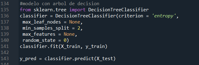
A confusion matrix is generated to verify the quality of the model

Confusion matrix results:

Based on the confusion matrix, we proceed to calculate the metrics that indicate the model's quality. We have the following:
TP = 273,905
FP = 2
FN = 2
TN = 26091
Accuracy = 0.9999
The accuracy is very good; however, as noted in the statistical analysis, fraud cases account for 8.7% of the data, resulting in an imbalanced dataset—that is, there is a large amount of data for one class (non-fraud) and very little for the other (fraud). Given this, we proceed to calculate the F1 score, which is the most appropriate metric for this type of case.
Precision = 0.9999
Recall = 0.9999
F1 score = 0.9999
It can be seen that the F1 score is very close to 1, so we can conclude that the model is of very high quality and will be highly effective in predicting future fraudulent transactions.
3. Random Forest
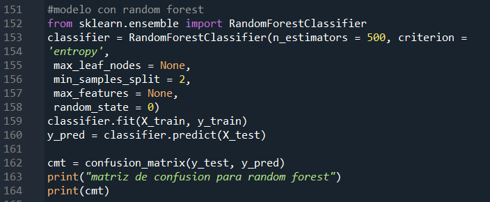
The results of the confusion matrix are displayed.

As you can see, it yields the same result as the decision tree.
4. K-nearest neighbors
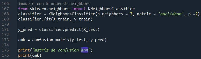
Confusion matrix results.
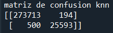
The table above shows that the quality of this model is lower than that of the model using the decision tree method. The model's evaluation metrics are calculated as follows:
TP = 273,713
FP = 194
FN = 500
TN = 25593
Accuracy = 0.9977
Precision = 0.9993
Recall = 0.9982
F1 score = 0.9987
5. Naive Bayes
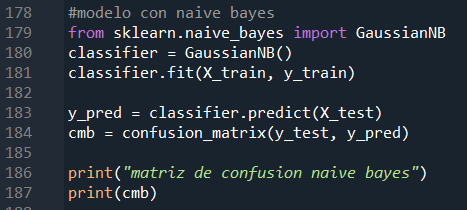
Confusion matrix results:
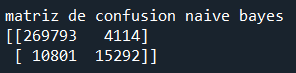
It can be seen that with this method, the model's quality declines even further compared to the previous models. The evaluation metrics are shown below:
TP = 269,793
FP = 4114
FN = 10801
TN = 15292
Accuracy = 0.9503
Precision = 0.9850
Recall = 0.9615
F1 score = 0.9731
6. Comparison of the Models
Finally, as a summary, a comparative table of the metrics for the different models used is provided, showing that the method with the best metrics—and therefore the one that should be used—is the decision tree, with an F1 score of 99.99%.

7. Clustering
Another important aspect of the business is categorizing transactions, by taking advantage of the benefits offered by machine learning and data mining We then proceed to perform the clustering. For this purpose, we worked with the numerical variables available in the dataset. As can be seen in the visualization (Power BI dashboard), the variables “distance from home” y “ratio relative to the average purchase price” These were the variables that showed the greatest variation in medians when fraud cases were analyzed separately from non-fraud cases; for this reason, these two variables are used in the clustering process.
The Elbow method is used to determine the optimal number of clusters.
The results of this method are shown below; as you can see, the number of clusters to use is 3.

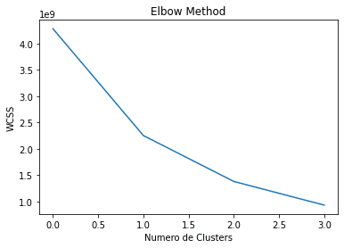
Figure 8. WCSS as a function of K (number of clusters).
Once the optimal number of clusters has been determined, we proceed to perform the clustering and create a graph to visualize the distribution of the data within each cluster:
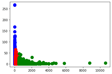
The graph shows a first cluster (blue) with transactions that are close to home but have a high ratio relative to the average purchase amount. In addition, there is a second cluster (red) with transactions that are at an average distance from home and have an average ratio relative to the average purchase amount. Finally, a third cluster (green) consists of transactions with a low ratio relative to the average purchase price and a high distance from home.
8. Conclusions
- The dataset card_transdata The data is of good quality in its original source, so it requires minimal processing for subsequent steps.
- 8.7% of the transactions under review are fraudulent.
- Result of the statistical study, It is determined that the variables “distance from home” and “same retailer” are correlated.
- With regard to fraud, it is determined that all the variables in the dataset are influential, except for the “same retailer” variable.
- In the correlation study It can be seen that the security measures adopted—such as the use of chips and PIN numbers—are effective in preventing fraud, as they show a negative correlation with fraud cases.
- Various models are developed using supervised learning methods to detect cases of fraud; the most effective model is the one that uses the decision tree method, with an F1 score of 99.99%; therefore, it is the the model that should be used.
- The transactions were categorized into 3 clusters, using the continuous variables “distance from home“ and ”ratio relative to the average purchase amount,” applying the elbow method to determine the optimal number of clusters, and using the K-Means algorithm for the clustering itself.
The Structuralia team would like to thank Magaly Fonseca for her excellent work. We wish her every success in her professional career and in all the challenges she takes on in the future!
AUTHOR'S REVIEW:
Magaly Fonseca Maroto, with a bachelor's degree in Industrial Production Engineering at the Technological Institute of Costa Rica. He also completed a technical certificate in computer networking and has taken courses in Six Sigma Green Belt, Customer Service, and PowerBI. He recently earned a Master's Degree in Big Data and Business Analytics in Structuralia.
He has been working for 12 years at ICE (Instituto Costarricense de Electricidad), Costa Rica’s state-owned electricity and telecommunications company, where he has led various technical teams and is responsible for preparing management reports for the department and participating in improvement projects.
AUTHOR'S STATEMENT:
1. Why did you choose Structuralia?
«I chose Structuralia because it was easy to study online. I found the curriculum to be very comprehensive and well-suited to my needs, and I was also able to apply for an OAS scholarship.".«
2. What would you highlight most about the master's program?
«What stands out to me about the Master’s in Big Data and Business Analytics is the breadth of topics covered. As a professional in industrial engineering without a strong background in computer science and programming, the way the program covers these topics allowed me to gain a deeper understanding and apply what I learned. I really appreciate that the methodology focuses on helping students gain a thorough understanding of each topic through a solid theoretical foundation combined with practical application, which is essential for internalizing what is covered in theory.”.
»In addition, the fact that students can work through the topics individually at their own pace is a major advantage of Structuralia. Combined with the user-friendly platform and the way it tracks the percentage of progress for each module and the master’s program as a whole, it’s very useful.".
3. How has it helped you, or how do you think it could help you, in your current or future professional development?
«Throughout my professional career, I have come to understand the importance of having access to data quickly, in a timely and effective manner, so that it can be transformed into information that enables robust and sound decision-making. This master’s program has helped me complement my career as an industrial engineer and enhance my skills with knowledge in Big Data and Business Analytics. Since these are rapidly growing fields, I am confident that the knowledge I have gained will open many doors for me to continue growing professionally and contribute to the development of the company where I work.».