
This master's thesis project optimizes time series forecasting using AI models. Discover advanced approaches to data analysis and decision-making.
Master's Thesis Project: Time Series Forecasting Using AI Models
This article focuses on the Final Project Master's Degree in Big Data and Business Analytics from our former student at the Daniel Cano Alvira, which seeks to explore the potential of artificial intelligence to predict movements in stock market indices with the goal of achieving positive returns in the financial markets. The project explores potential applications of artificial intelligence techniques in the field of investing, proposing and developing two possible approaches to address this challenge.
Objectives of the Master's Thesis
The objective of this study is to develop a price prediction model for use in financial markets. To this end, we will use Python in order to download the prices of various financial assets by connecting to Yahoo Finance. The code developed in this post will not be included so that it doesn't get too long.
Project Details
Yahoo Finance is an online service provided by Yahoo which offers a variety of financial information free of charge, including stock data, financial news, analysis tools, and resources for tracking markets and investments.
Although it does not have an official API, thanks to the large number of repositories available on GitHub Contribution data can be easily obtained. The repository that will be used is called yfinance, developed by Ran Aroussi, is the best alternative to Yahoo Finance, although it increasingly relies on outdated methods due to the website’s improved security against web scraping. For the purposes of this project, only the “Ticker” method will be used, and stock price data for certain stock indices will be downloaded from the Yahoo Finance global indices page using a very simple web scraping technique. A stock index is a figure calculated using an equation based on specific assets, with the aim of reflecting changes in value or returns of the assets that comprise it. The data will be returned as Japanese candlesticks; this type of data consists of four main components that describe the price movement of the underlying asset. These components are explained below, along with the rest of the data available in the resulting table.
- Date: Start date and time of the Japanese candlestick chart. When downloading daily candlestick charts, there will be one per day, so the date will be daily.
- Open (Opening): The asset's price at the start of the candlestick's time interval.
- High (Max): Highest price reached during the candle's time interval.
- Low (Minimum): Lowest quoted price during the candle's time interval.
- Close: The asset's price at the end of the candlestick's time interval.
- Volume: The number of contracts that have been transferred out of the total number of transactions carried out during the candle's time interval.
- Dividends: The amount of money paid per share to a company's shareholders. This applies only to stocks or ETFs.
- Stock Splits: The ratio multiplies the number of shares to increase or decrease the number available on the market. If it is less than one, it is considered a reverse split, in which the number of shares is reduced, usually with the goal of raising the price. If the ratio is greater than one, the number of shares increases, lowering the price and making them more affordable. This applies only to stocks and ETFs.
In our case, we will also calculate new data based on the data already mentioned in order to improve our predictive capabilities. The main ones are explained below.
- Range: The trading range for that candle is calculated by subtracting the low from the high.
- Range per unit: Price per unit is calculated by dividing the range by the opening price.
- Open to Close: The range between the opening and closing prices is calculated by subtracting the opening price (Open) from the closing price (Close). It is important to note that, unlike the Range, this figure will be negative when the price falls.
- Open to Close per unit: Range between the opening and closing prices, divided by the opening price (Open).
- Gap: The difference between the current opening price and the closing price of the previous candlestick.
- Gap per unit: The difference between the current opening price and the closing price of the previous candlestick, divided by the previous closing price.
- Moving Average difference per unit: The difference between the current opening price and the 10-, 20-, 50-, 100-, and 200-period moving averages.
- Weekday: The day of the week number (between 0 and 4) to which the candle corresponds.
Selection of the asset universe to be studied
Once the stock market indices had been web-scraped, it was decided to filter them due to their initial volume. By analyzing the time series of the various indices, it was concluded that the most actively traded are those in the U.S. market and that some indices have a daily range considerably smaller than others, such as the N225, IXIC, GSPC, and AORD. It is worth noting that the SPY has decent volume, sufficient volatility, and an appropriate price to enable efficient risk management in actual trading. Next, we will examine the correlation among the selected assets.
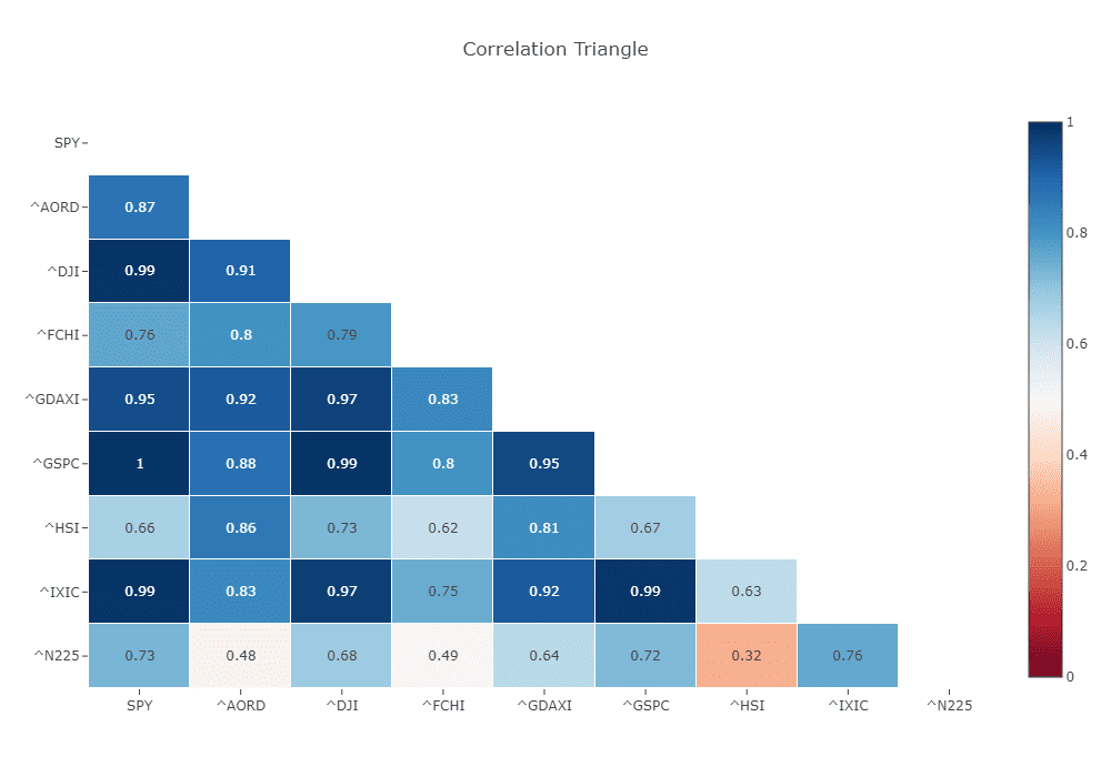
The figure shows the high correlation between them; the correlation is never negative and falls below 0.5 in only three cases. Since indices provide an overview of the direction and health of a particular segment of the financial market, when such an index represents a country’s top companies, its performance is generally considered to mirror the country’s economic health. If we combine this with the high correlation among indices from different countries, we might conclude that economic cycles are relatively synchronized, likely due to extensive globalization and international interdependence. We can deduce from all of this that the indices themselves likely have some predictive value relative to one another; this will be the hypothesis of the second case study to be conducted.
Strategy Evaluation Metrics
To validate the prediction systems, we will calculate industry-standard metrics as well as some that I personally believe may be interesting and help in understanding the system’s behavior. All of these metrics are based on past trades and are therefore purely indicative and subject to change over time.
1. Profitability
It measures performance in terms of net profit relative to invested capital. A positive return indicates that the system is generating profits.
Return on Investment = Net Income / Invested Capital × 100
2. Sharpe Ratio
It assesses the relationship between the additional return earned by taking on risk and the volatility of the portfolio. A high Sharpe ratio indicates a better risk-adjusted return. In practice, the yield on short-term government bonds, such as U.S. Treasury bills with maturities of three or six months, is commonly used as a proxy for the risk-free rate. This choice is based on the assumption that these bonds are relatively safe and liquid. Since this is beyond the scope of this study, we will use a risk-free rate of 0, which would be equivalent to keeping the money in a bank account.
Sharpe Ratio = Expected Return – Risk-Free Rate / Volatility × 100
3. Sortino Ratio
This metric is very similar to the Sharpe ratio, but instead of using the system's total volatility, it takes into account only the volatility of the negative positions.
Sortino Ratio = Expected Return – Risk-Free Rate / Negative Standard Deviation × 100
4. Maximum loss
It measures the largest decline in the portfolio balance from its peak. The smaller the decline, the greater the stability of the system.
Maximum Loss = (1 - Current Balance / Maximum Balance) × 100
5. Percentage of winning trades
The probability that any given trade will be profitable.
Probability of Winning = Number of Successful Trades / Total Number of Trades × 100
6. Risk-to-Return Ratio
It evaluates the relationship between gains and losses, helping to determine whether the system is generating returns that are proportionally greater than the risks taken.
Risk-Reward Ratio = Average Profit per Trade / Average Loss per Trade
7. Mathematical Expectation
It represents the weighted average of all possible outcomes of a random variable, taking into account the probability of each outcome occurring. In a financial context, expected value can be used to calculate the expected return on an investment, helping investors make informed decisions about where to allocate their resources.
Expected Value = (Probability of Winning * Average Profit per Trade –
Probability of Loss * Average Loss per Trade) × 100
Where: Probability of Losing = 1 - Probability of Winning
From the previous equation, we can understand the relationship between the probability of winning and the risk ratio. There will be a threshold beyond which the expected value is negative for every value of the probability of winning, since the lower the probability, the higher the return on investment must be relative to the loss (risk ratio) in order to remain profitable.
8. Kelly Size
A formula used in capital management theory and information theory to determine the optimal size of a series of bets. It is applicable in situations involving successive bets or investments and aims to maximize long-term capital growth. It is important to note that the Kelly Criterion is an aggressive strategy, and while it can maximize long-term growth, it can also lead to the loss of a large portion of capital in the short term if probability estimates are inaccurate.
Kelly = Probability of Winning - Probability of Losing / Risk-Reward Ratio × 100
9. Percentage of time in the market
The relationship between the number of days on which trades are executed and the number of days the system has been in use. A lower percentage is generally considered better, as it means less exposure to risk and lower commissions, if any maintenance fees apply.
Exposure Rate = Time with Open Positions / System Execution Time × 100
First Case Study
The first prediction attempt will involve applying an artificial intelligence model based solely on characteristics derived from the asset's own price. A comparison will be made of the application of the models:
- Linear Regression
- Logistic Regression
- K Nearest Neighbors (KNN)
- Naive Bayes
- Neural Network
- Random Forest
- Support Vector Machine (SVM)
Although the code for these models has been developed—rather than using the most common libraries—it will not be published so as not to make this post too long. If you would like access, please contact the author.
To avoid extending the project timeline, a minor optimization was performed before comparing the models. Below are three different graphs that will be used to compare the results from the training and test data, with the ultimate goal of identifying possible over-optimization.
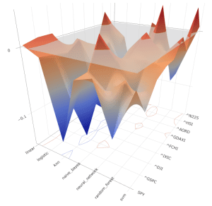
The first graph shows the variation in the probability of winning between the prediction results using test data and those using training data. It can be inferred that the closer the value is to 0, the less overfitting there is. The contour lines projected onto the lower plane show that the KNN model is the most overfitted of all, while the Linear Regression and Neural Network models are the least overfitted, even performing better with the test data than with the training data for some assets.
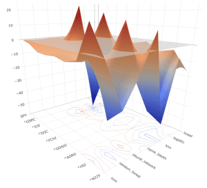
The following figure shows the difference in the expected value obtained from the training data and the test data. Since the probability of winning affects the expected value, it can be seen that the models in which this metric varies the least between the training and test data are the same as those in the previous graph. Although the Linear Regression model shows the least variation, when all assets are taken into account, the KNN model is once again the most overfitted, thus reaffirming the previous conclusion.
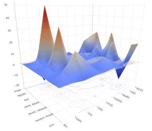
The Naive Bayes and KNN models have the lowest mean mathematical expectation, as shown in the following graph. It is worth noting that the Linear Regression, Neural Networks, and SVM models have the fewest features with a negative mathematical expectation, making them the most versatile. The results obtained by applying the PCA model to the features used have not been included, since they were worse than those obtained without applying it.
Finally, the changes in the balance sheet for each model will be calculated for each asset studied.
We will assume an initial capital of 100,000.01 TP4T and an allocation of 100 % to each of the models. Since risk management is beyond the scope of this study, we will trade using the total capital each time a trade is executed. Furthermore, only long positions will be considered, and commissions will be assumed to be zero. The figure shows a chart for each asset with the corresponding balance curve for each trained model. It can be seen that, in general, no single model stands out, but there are models that perform relatively well with U.S. indices, and it might be worth exploring them further and introducing risk management strategies.
It should be noted that only two years of data were used for the study, and that those years coincided with one year of recession and another marking the start of an expansion driven by central bank policies. It would be advisable to conduct a study using a larger dataset and to include a walk-forward test.
Second Case Study
The second exercise will involve predicting the prices of the SPY, an ETF that tracks the performance of the S&P 500. The idea behind this exercise is based on the time difference between various markets around the world. Since the Asian market has closed by the time the U.S. market opens, it stands to reason that the trading session on that day could be influenced by the performance of markets operating in earlier time zones. The data will be divided equally, with the first half serving as training data and the second half as the data to be predicted. Additionally, the same operational approach used in the previous exercise will be followed.
In this case, the models studied will be the following:
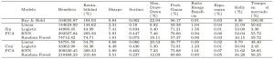
The following section presents a comparative analysis of the models based on the previously defined metrics. It can be seen that different models excel in different metrics, underscoring the importance of considering multiple criteria when evaluating financial strategies.
It has been decided to use the strategy of maintaining the total capital invested in the asset—commonly known as “Buy & Hold”—as a benchmark. For this strategy, a profit of 104,035.87$ is obtained, with a return of 104.03 %. The Sharpe ratio is 0.84, and the Sortino ratio is 0.062. Additionally, the maximum drawdown during the test period would be 22.94 %, and the probability of winning is 56.17 %. In general, the application of PCA does not appear to add value, with the Random Forest model being the sole exception. Although returns may be lower when using PCA, the reduction in dimensionality can be useful in terms of simplicity and computational efficiency. The Logistic Regression model yields the lowest return; this is due to its low trading frequency, with a market time of approximately 3 %. This, combined with its high reliability, makes it the model with the lowest maximum loss and the highest Sharpe ratio.
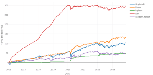
On the other hand, the K-Nearest Neighbors (KNN) model achieves the highest return, although this is due to overfitting. This occurs when the model is too closely fitted to the training data, resulting in patterns that are not well generalized. This can be seen in the figure above. During the first half (training), the capital increases steadily with almost no fluctuation, while in the test data, the capital fluctuates constantly between a maximum and a minimum.
The best strategy for your actual trading would be the Linear Regression model, to which you could incorporate the signals generated by the Logistic Regression model in order to achieve greater profits. In this specific case, the signals from the Logistic Regression model are also generated by the Linear Regression model, so they would not add any value unless they were taken into account in the risk management strategy.
The figure above compares the return and cumulative loss at each point in time for the final strategy and the “Buy & Hold” strategy. As you can see, the maximum loss is almost one-third that of “Buy & Hold,” while the strategy’s final return is 1.4 times that of “Buy & Hold.” All of this is achieved while entering the market only half as often.
Conclusions
The objective of this project was to study the feasibility of artificial intelligence models in predicting the prices of assets traded in financial markets. This project focused more on the models and their comparison than on capital and portfolio management. Although it has been demonstrated that, no matter how trendy artificial intelligence may be, it is not the holy grail, we have managed to develop strategies that may be worthwhile. In the first exercise, we observed that models often fail in their task if they are fed only with data derived from what we want to predict. Only in the most liquid markets did they achieve a certain degree of accuracy. The final exercise demonstrated the need to avoid overfitting models, as this can lead to disaster when applied to real-world trading. Furthermore, the importance of factor engineering in obtaining variables with greater predictive power has been highlighted. Artificial intelligence is part of our daily lives and has been applied in financial markets for decades. It will take a great deal of research and resources to develop a system capable of matching the returns of industry leaders such as Medallion Fund.
In the future, it would be advisable to include operational and capital management, since there are many variables that depend on these factors and have been assumed in this study. Some ideas to start with could be: adding stop-loss and take-profit limits to positions instead of keeping them open all day, and defining an algorithm to allocate the percentage of the account to risk at any given time. On the other hand, it would be advisable to define the time interval for retraining the model, since keeping the model up to date requires training it with new data. It would be necessary to define how often the model should be retrained and the amount of data to be used, since past patterns may contradict current ones and impair the model’s predictive ability.

Author's Review
Daniel Cano, holds a degree in Energy Engineering from the Polytechnic University of Madrid and has recently completed the Master's Degree in Big Data and Business Analytics. He currently works at Técnicas Reunidas S.A., specifically in the Digital Transformation department. Daniel has his own personal project page, «One Made«.
Author's Testimony
1. Why did you choose Structuralia?
«My company gave me the opportunity to further my education and specialize by pursuing a master's degree. When I had to choose among several options, the master's program at Structuralia was the one that appealed to me the most.»
2. What would you highlight most about the master's program?
«What I would highlight most is that the Master's in Big Data and Business Analytics provides excellent documentation and materials.»
3. How has it helped you, or how do you think it could help you, in your current or future professional development?
«Completing this master's program has helped me better understand and reinforce concepts I already knew. I've also been able to learn about new Big Data tools.«